
We begin by converting the image to grayscale since we rely on the distinct shape of the fiducial markers, not their specific color. This is done with OpenCV’s cvtColor() function.
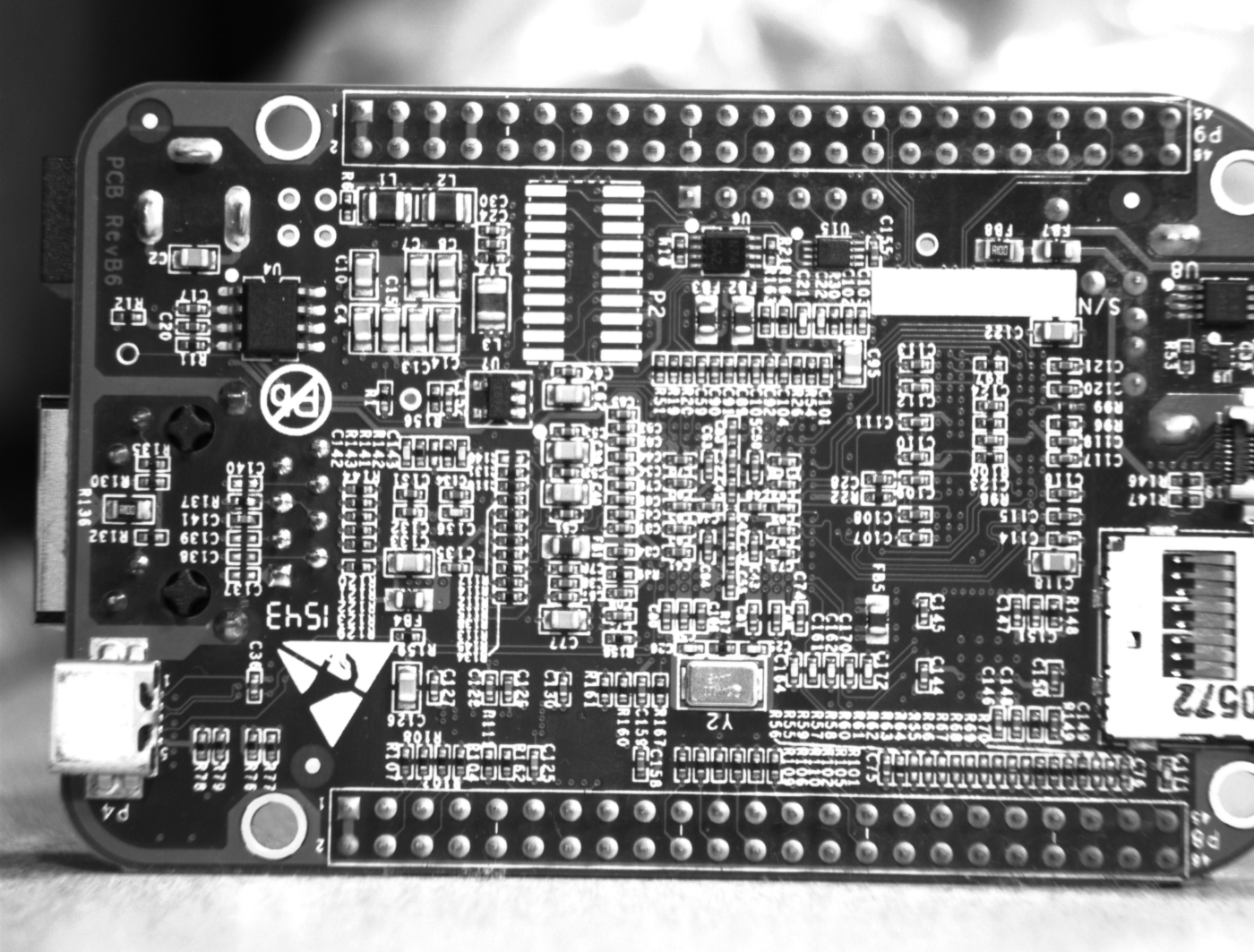
The fiducial markers on this PCB are composed of two concentric disks whose respective diameters are 26 and 68 pixels.
OpenCV’s matchTemplate() function requires a template image of the target object. In this case, it would be an image of a fiducial marker. We could crop one of the three fiducial markers in our image and use it as our template, but this approach is prone to missing true fiducial markers that have minor appearance differences with the arbitrarily chosen template image. Instead, we’ll create a synthetic image of an ideal fiducial marker:
The fiducial marker image is standardized to zero mean and unity standard deviation because we want the result of matchTemplate() to be close to zero in areas of uniform values in the searched image, and the intensity values of the positive matches to be close to 1.
We now have all the ingredients needed to call matchTemplate():
It is important to note that we padded the resulting matched image with zeros, to have an image that has the same dimensions as the original image. It is necessary because, matchTemplate() being based on convolution, the output image has dimensions (Wₒᵣᵢ-Wₚₐₜₜₑᵣₙ+1, Hₒᵣᵢ-Hₚₐₜₜₑᵣₙ+1). In our case, the pattern image having dimensions (69, 69), the output of matchTemplate() has dimensions 68 pixels narrower and 68 pixels shorter than the original image. To compensate for this effect, we zero-padded 34 pixels in the image periphery. We also rescaled the gray levels of the matched image, from [-1, 1] to [0, 255] to visualize it easily.
We are interested in the peaks in the intensity of the matched image, represented by bright spots in the above image. Deciding which bright spots are the fiducial markers we are searching for is a matter of setting the right threshold.
Instead of setting the threshold manually, we’ll use the fact that we know there should be three fiducial markers in this match image, and therefore applying the right threshold should result in a binary image with exactly three blobs¹. To do that, we’ll gradually lower the threshold, starting from 255 and counting the blobs in the resulting thresholded images. When we reach three blobs, we stop.
Three correspondences between reference points on the PCB plane (in millimeters) and their respective locations in the image (in pixels) is the minimum needed to compute a homography, i.e. the transformation matrix that allows us to convert coordinates in millimeters to coordinates in pixels. Using this transformation matrix, we can annotate the image with the PCB edges.
The annotated image above confirms that the three fiducial markers were correctly found and the computed transformation matrix is accurate. It is now possible to crop any area of the image where there should be a given component that we want to inspect, assuming we have its physical coordinates on the PCB.
In a manufacturing environment, it is common that the objects to be inspected are moving on a conveyor. We cannot assume that the object to be inspected will always be precisely located at the same place relative to the camera. The transformation matrix computed from the detection of the fiducial markers allows us to retrieve a given area of interest on the PCB even if there is a translation and a rotation from one object to the next.