To create a cartoon effect, we need to pay attention to two things; edge and color palette. Those are what make the differences between a photo and a cartoon. To adjust that two main components, there are four main steps that we will go through:
- Load image
- Create edge mask
- Reduce the color palette
- Combine edge mask with the colored image
Before jumping to the main steps, don’t forget to import the required libraries in your notebook, especially cv2 and NumPy.
import cv2
import numpy as np# required if you use Google Colab
from google.colab.patches import cv2_imshow
from google.colab import files
The first main step is loading the image. Define the read_file function, which includes the cv2_imshow to load our selected image in Google Colab.
Call the created function to load the image.
uploaded = files.upload()
filename = next(iter(uploaded))
img = read_file(filename)
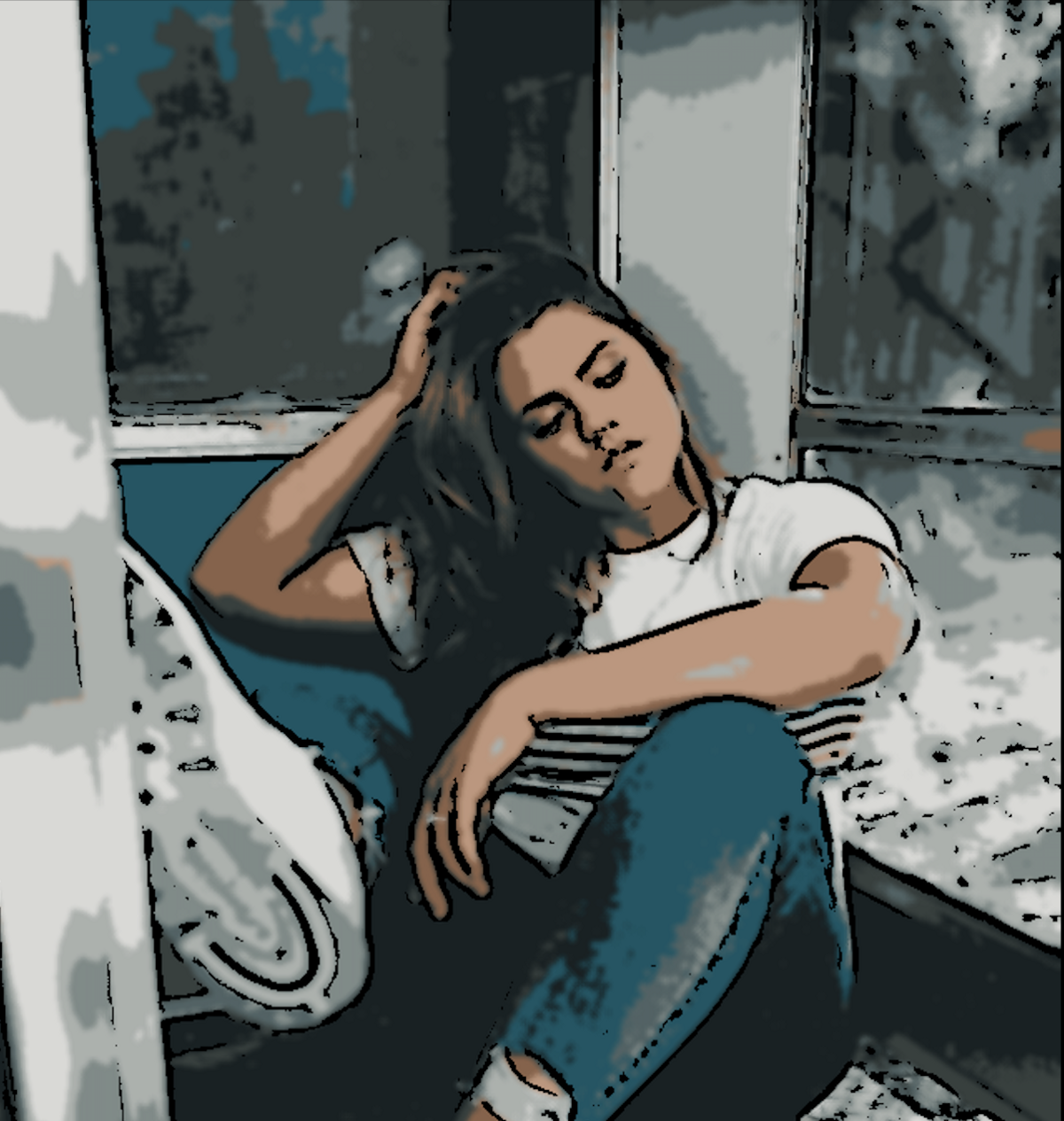
I chose the image below to be transformed into a cartoon.
Commonly, a cartoon effect emphasizes the thickness of the edge in an image. We can detect the edge in an image by using the cv2.adaptiveThreshold() function.
Overall, we can define the egde_mask function as:
In that function, we transform the image into grayscale. Then, we reduce the noise of the blurred grayscale image by using cv2.medianBlur. The larger blur value means fewer black noises appear in the image. And then, apply adaptiveThreshold function, and define the line size of the edge. A larger line size means the thicker edges that will be emphasized in the image.
After defining the function, call it and see the result.
line_size = 7
blur_value = 7edges = edge_mask(img, line_size, blur_value)
cv2_imshow(edges)
The main difference between a photo and a drawing — in terms of color — is the number of distinct colors in each of them. A drawing has fewer colors than a photo. Therefore, we use color quantization to reduce the number of colors in the photo.
Color Quantization
To do color quantization, we apply the K-Means clustering algorithm which is provided by the OpenCV library. To make it easier in the next steps, we can define the color_quantization function as below.
We can adjust the k value to determine the number of colors that we want to apply to the image.
total_color = 9
img = color_quantization(img, total_color)
In this case, I used 9 as the k value for the image. The result is shown below.
Bilateral Filter
After doing color quantization, we can reduce the noise in the image by using a bilateral filter. It would give a bit blurred and sharpness-reducing effect to the image.
blurred = cv2.bilateralFilter(img, d=7, sigmaColor=200,sigmaSpace=200)
There are three parameters that you can adjust based on your preferences:
- d — Diameter of each pixel neighborhood
- sigmaColor — A larger value of the parameter means larger areas of semi-equal color.
- sigmaSpace –A larger value of the parameter means that farther pixels will influence each other as long as their colors are close enough.
The final step is combining the edge mask that we created earlier, with the color-processed image. To do so, use the cv2.bitwise_and function.
cartoon = cv2.bitwise_and(blurred, blurred, mask=edges)
And there it is! We can see the “cartoon-version” of the original photo below.